m Change the layout a bit. |
m Change where the first image is. |
||
| Line 25: | Line 25: | ||
This term shows that hit chance decreases the further the target is beyond optimal range. This relationship can be visualized along a 1D axis. | This term shows that hit chance decreases the further the target is beyond optimal range. This relationship can be visualized along a 1D axis. | ||
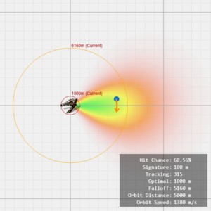
[[File:Turret tracking visualization.png|thumb|alt=The heatmap of hit chance, from a stationary 200mm Autocannon I without any ammo or skill, tracking an orbitting object at a distance of 5000 meter and 1380m/s speed, is 60.55%.|The heatmap of hit chance, from a stationary 200mm Autocannon I without any ammo or skill, tracking an orbitting object.]] | |||
Next, consider the tracking term: | Next, consider the tracking term: | ||
| Line 38: | Line 41: | ||
From this, we can interpret the turret's tracking stat as a kind of '''"maximum allowable angular velocity"''' it can handle. Visually, this forms a 2D cone shape where hit chance remains high within the cone and falls off outside of it. | From this, we can interpret the turret's tracking stat as a kind of '''"maximum allowable angular velocity"''' it can handle. Visually, this forms a 2D cone shape where hit chance remains high within the cone and falls off outside of it. | ||
Revision as of 15:05, 30 May 2025
This will be the personal draft space for elaborating the idea.
Widget will be released on github or something...
Visualization formula derivation
It is recommended to read the Turret_mechanics#Hit_chance section beforehand, as this explanation assumes a basic understanding of turret mechanics.
According to the hit chance formula, we have:
To visualize this complex formula intuitively, we apply the following constraints to simplify the setup:
- The attacker is stationary.
- The target is either stationary or moving in a perfect circular orbit around the attacker.
- The scenario takes place on a 2D plane.
First, consider the distance term.
This term shows that hit chance decreases the further the target is beyond optimal range. This relationship can be visualized along a 1D axis.

Next, consider the tracking term:
We can visualize the target's orbiting motion as an arc. The length of this arc over one second represents the target’s orbital velocity. For a given orbital velocity, the angular velocity (how quickly the target moves across the turret’s aim) increases as the orbital radius (distance to the attacker) decreases:
This means: the closer the target is while orbiting at the same speed, the harder it is for the turret to track.
From this, we can interpret the turret's tracking stat as a kind of "maximum allowable angular velocity" it can handle. Visually, this forms a 2D cone shape where hit chance remains high within the cone and falls off outside of it.
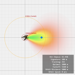
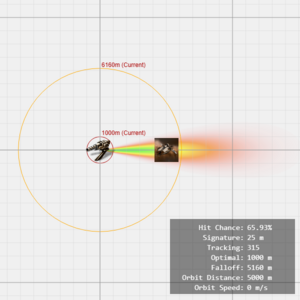
By combining the 1D distance-based falloff term with the 2D angular velocity-based tracking cone, we can visualize the hit chance on a 2D plane using a heatmap.
Title for some examples ?
Examples for parameters change and practical usage (web, TP, tracking computer etc.)
Title 2
|
|
|
|
|---|
|
|
|
|
|---|
|
|
|
|
|---|
Title 3
Some more description...
Some more description...
Some more description...


